Students can download 12th Business Maths Chapter 9 Applied Statistics Ex 9.1 Questions and Answers, Samacheer Kalvi 12th Business Maths Book Solutions Guide Pdf helps you to revise the complete Tamilnadu State Board New Syllabus and score more marks in your examinations.
Tamilnadu Samacheer Kalvi 12th Business Maths Solutions Chapter 9 Applied Statistics Ex 9.1
Question 1.
Define Time series.
Solution:
When quantitative data are arranged in the order of their occurrence, the resulting series is called the Time Series.
Question 2.
What is the need for studying time series?
Solution:
We should study time series for the following reasons.
- It helps in the analysis of past behaviour.
- It helps in forecasting and for future plans.
- It helps in the evaluation of current achievements.
- It helps in making comparative studies between one time period and others.
Therefore time series helps us to study and analyze the time-related data which involves in business fields, economics, industries, etc…
![]()
Question 3.
State the uses of time series.
Solution:
A time-series carries profound importance in business and policy planning. It is used to compare the current trends with that in the past or the expected trends. Thus it gives a clear picture of growth or downfall. Most of the time series data related to fields like Economics, Business, Commerce etc. For example the production of a product, cost of a product, sales of a product, national income, salary of an individual etc. By close observation of time series data, one can predict and plan for future operations in industries and other fields.
Question 4.
Mention the components of the time series.
Solution:
Components of Time Series
There are four types of components in a time series. They are as follows;
- Secular Trend
- Seasonal variations
- Cyclic variations
- Irregular variations
![]()
Question 5.
Define the secular trend.
Solution:
Secular Trend: It is a general tendency, of time series to increase or decrease or stagnates during a long period of time. An upward tendency is usually observed in the population of a country, production, sales, prices in industries, the income of individuals etc., A downward tendency is observed in deaths, epidemics, prices of electronic gadgets, water sources, mortality rate etc….
Question 6.
Write a brief note on seasonal variations.
Solution:
Seasonal Variations: As the name suggests, tendency movements are due to nature which repeats themselves periodically in every season. These variations repeat themselves in less than one year time. It is measured in an interval of time. Seasonal variations may be influenced by natural force, social customs and traditions. These variations are the results of such factors which uniformly and regularly rise and fall in the magnitude. For example, selling of umbrellas’ and raincoat in the rainy season, sales of cool drinks in the summer season, crackers in Deepawali season, purchase of dresses in a festival season, sugarcane in Pongal season.
![]()
Question 7.
Explain cyclic variations.
Solution:
Cyclic Variations: These variations are not necessarily uniformly periodic in nature. That is, they may or may not follow exactly similar patterns after equal intervals of time. Generally, one cyclic period ranges from 7 to 9 years and there is no hard and fast rule in the fixation of years for a cyclic period. For example, every business cycle has a Start- Boom-Depression- Recover, maintenance during booms and depressions, changes in government monetary policies, changes in interest rates.
Question 8.
Discuss irregular variation.
Solution:
Irregular Variations: These variations do not have a particular pattern and there is no regular period of time of their occurrences. These are accidental changes which are purely random or unpredictable. Normally they are short – term variations, but its occurrence sometimes has its effect so intense that they may give rise to new cyclic or other movements of variations. For example floods, wars, earthquakes, Tsunami, strikes, lockouts etc…
![]()
Question 9.
Define the seasonal index.
Solution:
Seasonal Index for every season (i.e) months, quarters or year is given by
Seasonal Index (S.I) = \(\frac{\text { Seasonal Average }}{\text { Grand average }}\) × 100
Where seasonal average is calculated for month, (or) quarter depending on the problem and Grand Average (G) is the average of averages.
Question 10.
Explain the method of fitting a straight line.
Solution:
The method of fitting a straight line is as follows
Procedure:
(i) The straight-line trend is represented by the equation Y = a + bX ….. (1)
where Y is the actual value, X is time, a, b are constants
(ii) The constants ‘a’ and ‘b’ are estimated by solving the following two normal Equations
ΣY = n a + b ΣX ……(2)
ΣXY = a ΣX + b ΣX2 ……(3)
Where n = number of years given in the data.
(iii) By taking the mid-point of the time as the origin, we get ΣX = 0
(iv) When ΣX = 0, the two normal equations reduces to
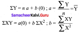
The constant ‘a’ gives the mean of Y and ‘6’ gives the rate of change (slope).
(v) By substituting the values of ‘a’ and ‘b’ in the trend equation (1), we get the Line of Best Fit.
![]()
Question 11.
State the two normal equations used in fitting a straight line.
Solution:
The normal equations used in fitting a straight line are
ΣY = na + b ΣX and ΣXY = a ΣX + b ΣX2
Where n = number of years given in the data,
X = time
Y = actual value
a, b = constants
Question 12.
State the different methods of measuring trend.
Solution:
Measurements of Trends
Following are the methods by which we can measure the trend.
- Freehand or Graphic Method
- Method of Semi-Averages
- Method of Moving Averages
- Method of Least Squares
![]()
Question 13.
Compute the average seasonal movement for the following series.
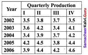
Solution:
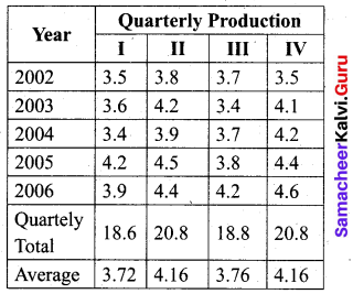
Grand average = \(\frac{3.72+4.16+3.76+4.16}{4}\) = 3.95
Seasonal Index (S.I) for I quarter = \(\frac { Average\quad of\quad I\quad quarter }{ Grand\quad Average }\) × 100
S.I. for I quarter = \(\frac{3.72}{3.95}\) × 100 = 94.1772
S.I. for II quarter = \(\frac{4.16}{3.95}\) × 100 = 105.3165
S.I. for III quarter = \(\frac{3.76}{3.95}\) × 100 = 95.1899
S.I. for IV quarter = \(\frac{4.16}{3.95}\) × 100 = 105.3165
Thus we obtain the average seasonal movement.
Question 14.
The following figures relate to the profits of a commercial concern for 8 years.

Find the trend of profits by the method of three year moving averages.
Solution:
Computation of three-yearly moving averages
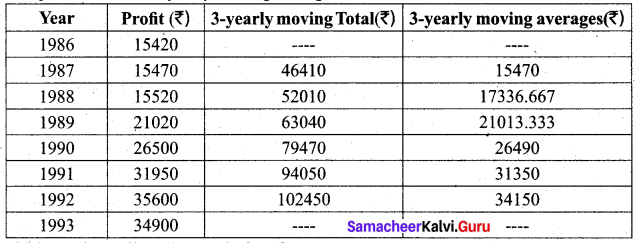
The last column gives the trend of profits.
![]()
Question 15.
Find the trend of production by the method of a five-yearly period of moving average for the following data:
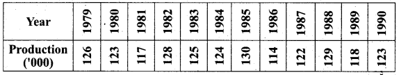
Solution:
Computation of five-yearly moving averages
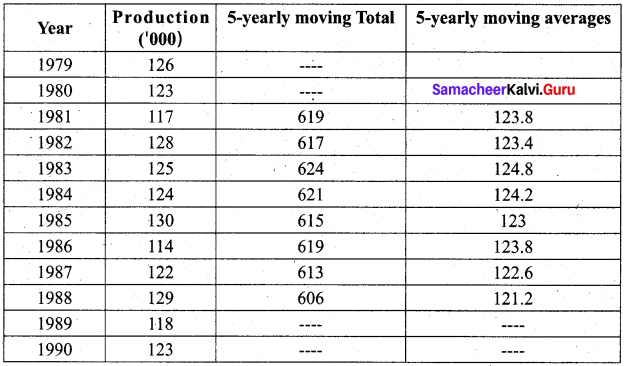
The last column gives the trend in the production by the method of the five-yearly period of moving average.
Question 16.
The following table gives the number of small – scale units registered with the Directorate of Industries between 1985 and 1991. Show the growth on a trend line by the freehand method.
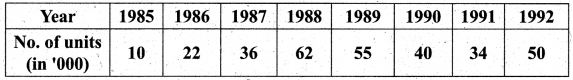
Solution:
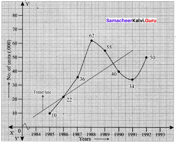
We follow the procedure as given below
(a) Plot the data on a graph
(b) Join all the points by a free hand smooth curve
(c) A line is drawn which passes through the maximum number of plotted points
![]()
Question 17.
The Annual production of a commodity is given as follows:
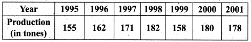
Fit a straight line trend by the method of least squares.
Solution:
Computation of trend values by the method of least squares. (ODD years)
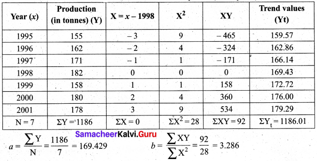
Therefore, the required equation of the straight line trend is given by Y = a + bX
(i.e) Y = 169.429 + 3.286 X (or) Y = 169.429 + 3.286 (x – 1998)
The trends values are obtained by
When x = 1995, Yt = 169.429 + 3.286 (1995 – 1998) = 159.57
When x = 1996, Yt = 169.429 + 3.286 (1996 – 1998) = 162.86
When x = 1997, Yt = 169.429 + 3.286 (1997 – 1998) = 166.14
When x = 1998, Yt = -169.429 + 3.286 (1998 – 1998) = 169.43
When x = 1999, Yt = 169.429 + 3.286 (1999 – 1998) = 172:72
When x = 2000, Yt = 169.429 + 3.286 (2000 – 1998) = 176.00
When x = 2001, Yt = 169.429 + 3.286 (2001 – 1998) = 179.29
Question 18.
Determine the equation of a straight line which best fits the following data.
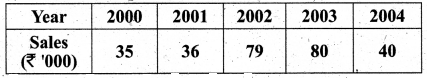
Compute the trend values for all years from 2000 to 2004.
Solution:
Computation of trend values by the method of least squares. (ODD years)
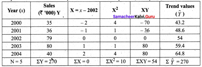
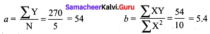
Therefore, the equation of the straight line which best fits the data is given by Y = a + b X
(i.e) Y= 54 + 5.4 X
(or) Y = 54 + 5.4 (x – 2002)
The trends values are obtained as follows
When x = 2000, \(\hat{Y}\) = 54 + 5.4 (2000 – 2002) = 43.2
When x = 2001, \(\hat{Y}\) = 54 + 5.4 (2001 – 2002) = 48.6
When x = 2002, \(\hat{Y}\) = 54 + 5.4 (2002 – 2002) = 54
When x = 2003, \(\hat{Y}\) = 54 + 5.4 (2003 – 2002) = 59.4
When x = 2004, \(\hat{Y}\) = 54 + 5.4 (2004 – 2002) = 64.8
![]()
Question 19.
The sales of a commodity in tones varied from January 2010 to December 2010 as follows:
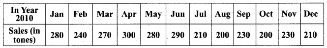
Fit a trend line by the method of semi-average.
Solution:
Since the number of months is even (12), we can equally divide the given data in two equal parts and obtain the averages of the first six months and last six months
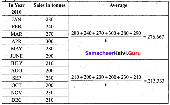
Thus we obtain semi-average I = 276.667 and semi-average II = 213.333
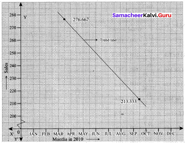
To fit a trend line we plot each value at the mid-point (month) of each half, (i.e) we plot 276.667 in the middle of March and April; we plot 213.333 in the middle of September and October. We join the two points by a straight line. This is the required line.
Question 20.
Use the method of monthly averages to find the monthly indices for the following data of production of a commodity for the years 2002, 2003 and 2004.
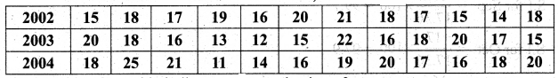
Solution:
Computation of monthly indices for the production of a commodity using the method of monthly averages.
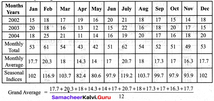
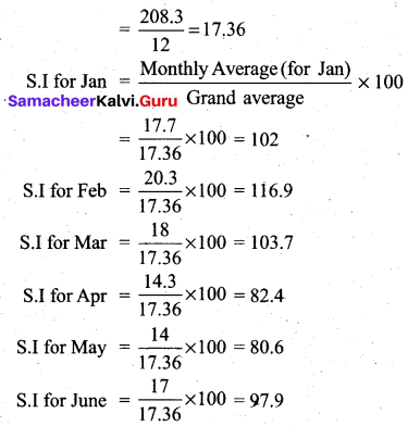
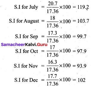
All the values are given in the above table in the last row.
![]()
Question 21.
Calculate the seasonal indices from the following data using the average from the following data using the average method:
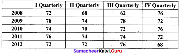
Solution:
Computation of quarterly indices.by the method of simple averages.
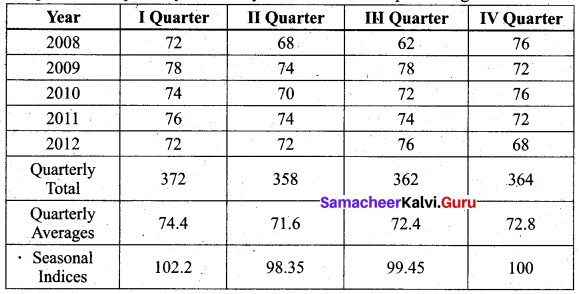
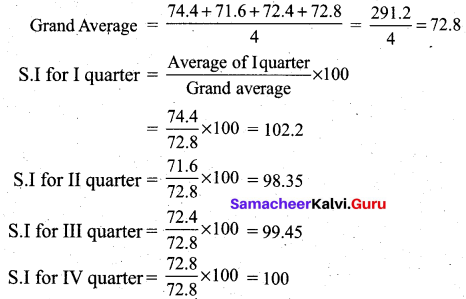
The seasonal indices are given in the last row of the table above.
Question 22.
The following table shows the number of salesmen working for a certain concern.
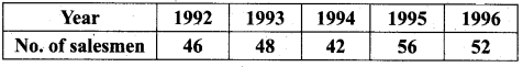
Use the method of least squares to fit a straight line and estimate the number of salesmen in 1997.
Solution:
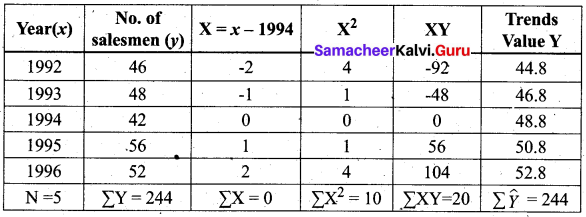
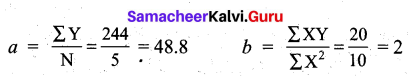
Therefore, the required equation of the straight line trend is given by
Y = a + bX
Y = 48.8 + 2 X
Y = 48.8 + 2 (x – 1994)
The trend values are obtained as follows:
When x = 1992, \(\hat{Y}\) = 48.8 + 2(1992 – 1994) = 44.8
When x = 1993, \(\hat{Y}\) = 48.8 + 2 (1993 – 1994) = 46.8
When x = 1994, \(\hat{Y}\) = 48.8 + 2 (1994 – 1994) = 48.8
When x = 1995, \(\hat{Y}\) = 48.8 + 2 (1995 – 1994) = 50.8
When x = 1996, \(\hat{Y}\) = 48.8 + 2 (1996 – 1994) = 52.8
In the year 1997, the estimated number of salesmen is \(\hat{Y}\) = 48.8 + 2 (1997 – 1994)
= 48.8 + 6
= 54.8 ~ 55